Decomposing the drivers of polar amplification with a single column model.

I submitted the last paper from my PhD onto EarthArXiv: Decomposing the drivers of polar amplification with a single column model, done in collaboration with Tim Merlis, Nick Lutsko, and Brian Rose. Here is a summary of the motivation of the paper and the main result.

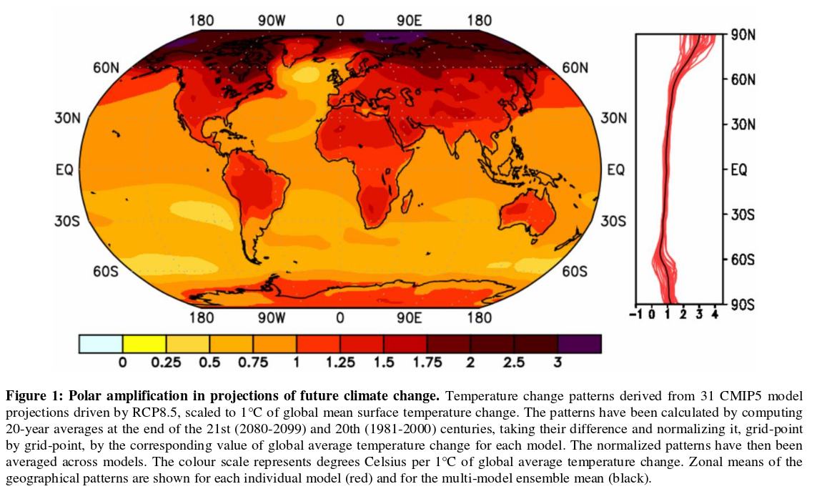
The work is focused on understanding the causes of polar amplification: the warming from increasing greenhouse gases is amplified at high latitudes both in models and observations.

Top-of-atmosphere budget analysis

Various mechanisms are thought to contribute to polar amplification: sea-ice albedo feedback, lapse rate and Planck feedback, atmospheric and oceanic heat transport changes. There generally has been two approaches to investigate the contributions of each of them. The first is to turn a certain mechanism off and see how that affects the pattern of warming $($mechanism denial experiment$)$. The second method is to diagnose how each mechanism contributes to the pattern of warming through some kind of budget analysis.

Pithan and Mauritsen (2014) quantify the contributions of various forcings and feedbacks to polar amplification in CMIP5 models using a top-of-atmosphere energy budget based method described below. In the figure below, the distance from the one-to-one line determines how much this forcing or feedback contributes to Arctic / tropical amplification.

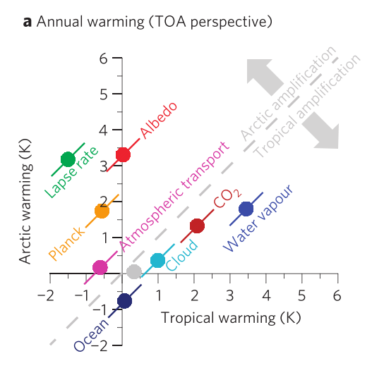
They use radiative kernels to figure out how each change $($increase in water vapour, decrease in Arctic sea ice, increase in equator-to-pole atmospheric energy transport, etc$)$ affects the top-of-atmosphere energy budget. The amount of surface temperature change is then derived by assuming that a vertically uniform surface and atmospheric temperature change balances the given top-of-atmosphere energy imbalance. For example, we know that the CO2 forcing and water vapor feedback are tropically amplified, hence they contribute to tropical amplification in the figure above. Any deviation from vertically uniform warming is then accounted for in the lapse rate feedback term, which becomes a dominant cause of polar amplification.

Forcing dependence of high latitude lapse rate feedback

In a simple analytical model of the Arctic atmosphere, Cronin and Jansen (2016) found that the high latitude lapse rate change depends on the forcing. The figure below shows how the high latitude temperature varies when the longwave optical depth $($a$)$, the surface forcing $($b$)$, and the atmospheric forcing $($c$)$ are varied. This breaks the linearity between surface temperature change and top-of-atmosphere radiation, i.e. when forced with a change in longwave optical depth $($CO2 or water vapor$)$, the surface temperature changes more for a given top-of-atmosphere radiation change than if forced with a change in atmospheric energy transport.

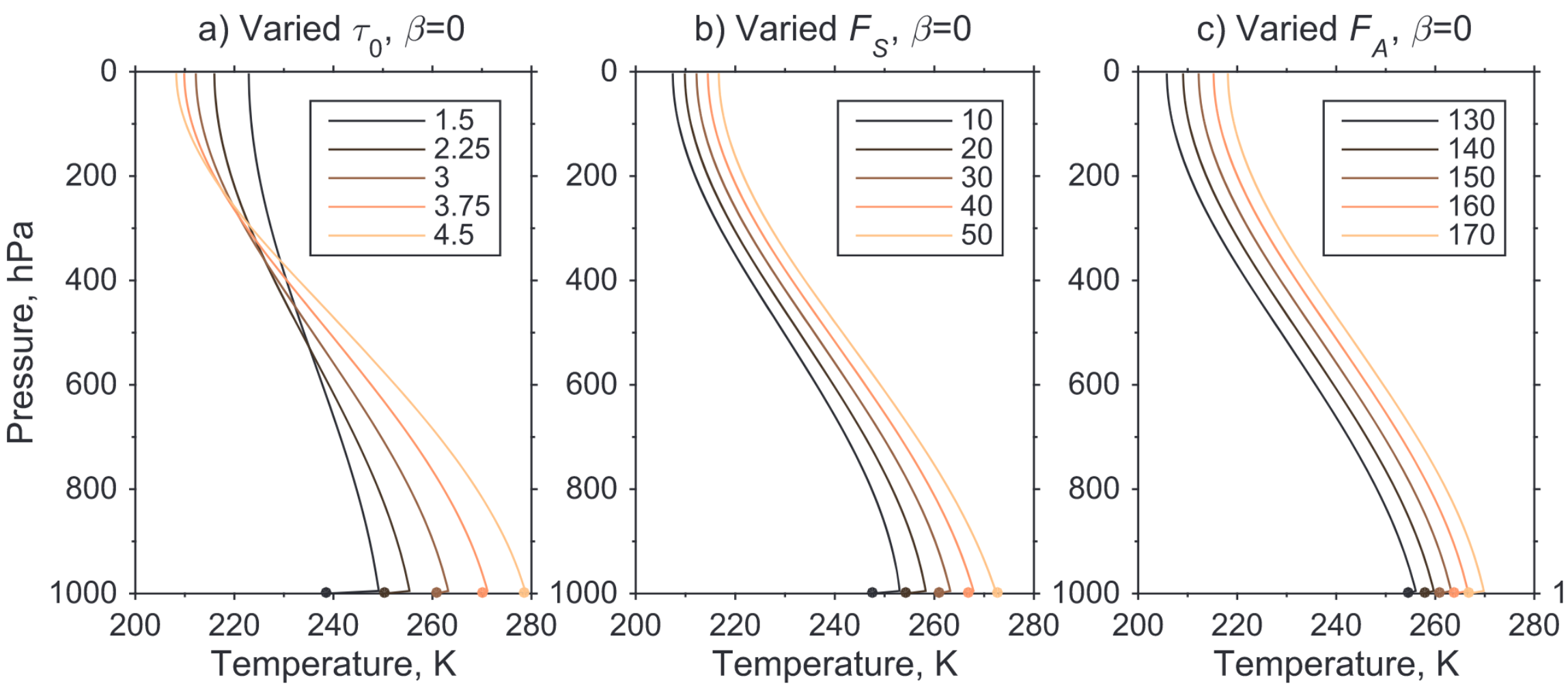
By assuming that top-of-atmosphere radiation imbalances are balanced by vertically uniform surface and atmosphere temperature changes, the top-of-atmosphere budget analysis does not account for how various forcings and feedbacks affect the high latitude lapse rate differently.

Single column model attribution method

The objective of this paper is to attribute the pattern of surface temperature change to the various forcings and feedbacks using a single column model in order to account for the forcing dependence of lapse rate change.

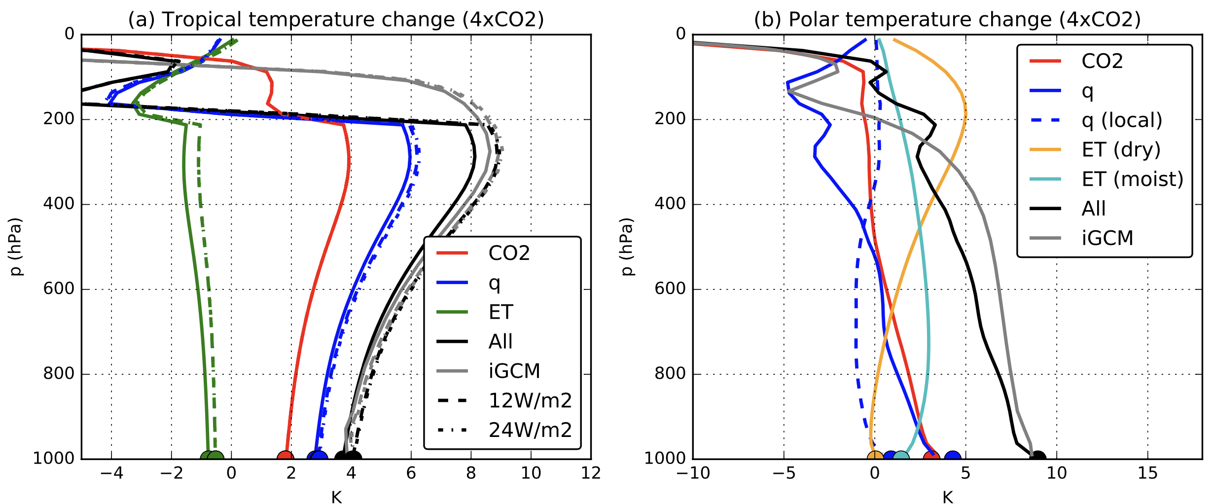
I first run a warming experiment in an idealized GCM $($aquaplanet, no clouds, no sea ice, comprehensive radiation, similar setup to MiMA$)$. The figure above shows the tropical $($a$)$ and polar temperature change $($b$)$ of the idealized GCM in grey. It is then decomposed using the single column model into the effects of just CO2 $($red$)$, water vapor $($blue$)$, and energy transport $($green for tropics and separated into dry and moist for polar region$)$. The single column model is used to best emulate the idealized GCM. In black, the temperature change when all the parameters are changed matches the idealized GCM temperature change, in grey, well enough.

In the tropics, the atmosphere is in radiative-convective equilibrium, hence the temperature structure of the atmosphere is close to moist adiabatic. Any perturbation leads to roughly the same vertical temperature change structure.

At high latitudes, the vertical structure of temperature change depends on the forcing. As predicted by the simple Cronin and Jansen model, the increase in longwave optical depth $($CO2 and water vapor$)$ leads to surface-enhanced warming. The increase in energy transport however has a more complex vertical structure. This is expected as the parametrization of energy transport in the Cronin and Jansen model was simplistic.

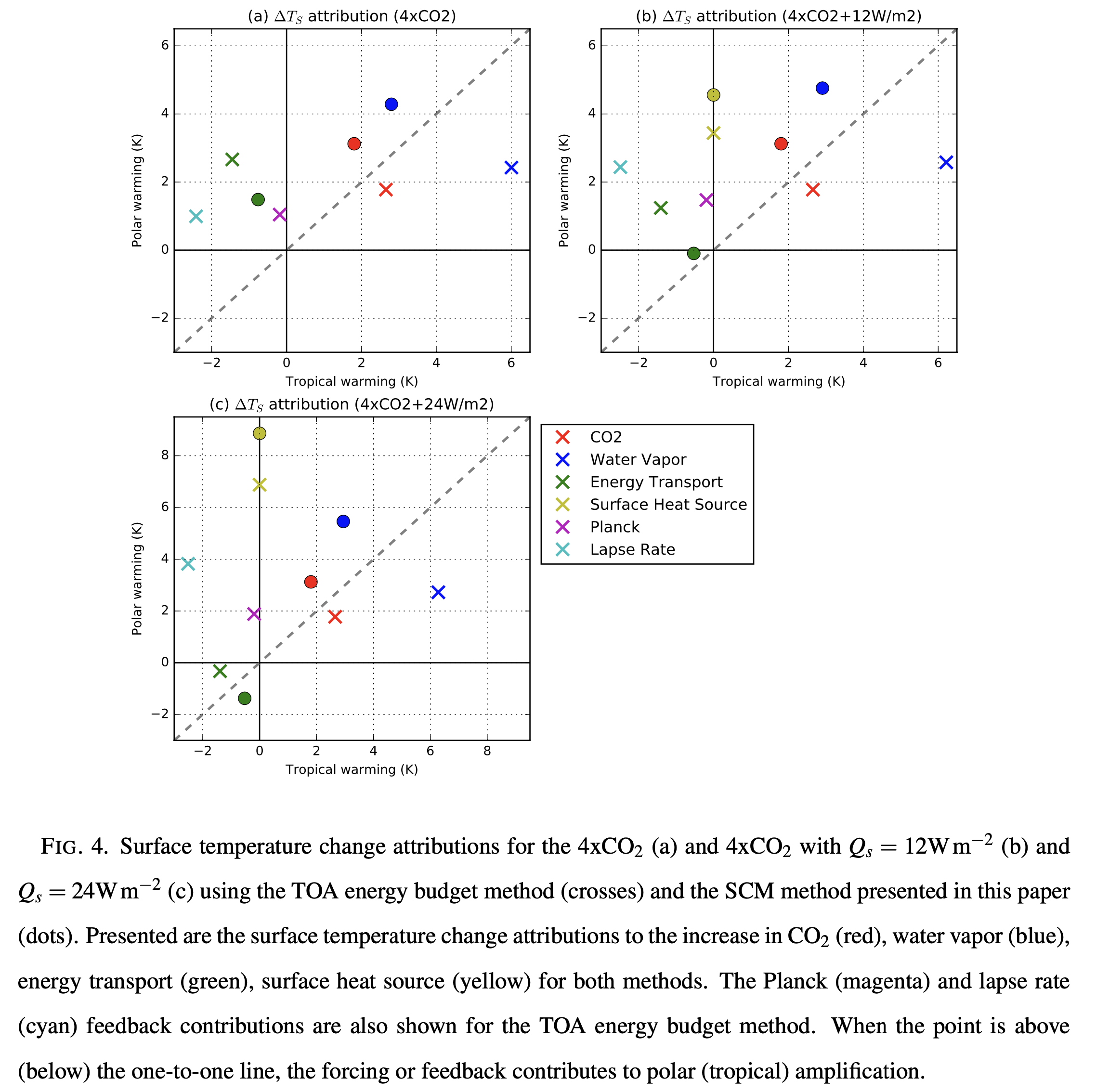
In the figure above, we compare the attribution based on the single column model $($dots$)$ and an attribution based on top-of-atmosphere energy imbalance, like in Pithan and Mauritsen $($crosses$)$. A surface heat source is applied at high latitudes $($12 W/m2 $($b$)$ and 24 W/m2 $($c$)$$)$ to simulate the effect of local feedbacks $($such as the sea-ice albedo feedback$)$. As in Pithan and Mauritsen, the lapse rate, Planck, and sea-ice albedo / local surface heat source are the main contributors to polar amplification.

In the single column model attribution $($dots$)$ however, CO2 and water vapor contribute to polar amplification due to their surface-enhanced warming structures at high latitudes and the presence of convection in low latitudes. The polar warming structure from atmospheric energy transport convergence is reduced as it preferentially warms the mid and upper troposphere.

Conclusion

In conclusion, this work comes as a follow-up to Pithan and Mauritsen’s influential paper on polar amplification. The explanation that the lapse rate feedback causes polar amplification was unsatisfactory as the lapse rate feedback, at high latitudes, is not a single process but a result of how the various forcings and feedbacks affect the vertical structure of temperature change. This single column model enables us to separate the drivers of vertical temperature change at high latitudes and get a clearer picture of the drivers of polar amplification.